Julian PT Higgins, Tianjing Li, Jonathan J Deeks
Key Points:
- The types of outcome data that review authors are likely to encounter are dichotomous data, continuous data, ordinal data, count or rate data and time-to-event data.
- There are several different ways of comparing outcome data between two intervention groups (‘effect measures’) for each data type. For example, dichotomous outcomes can be compared between intervention groups using a risk ratio, an odds ratio, a risk difference or a number needed to treat. Continuous outcomes can be compared between intervention groups using a mean difference or a standardized mean difference.
- Effect measures are either ratio measures (e.g. risk ratio, odds ratio) or difference measures (e.g. mean difference, risk difference). Ratio measures are typically analysed on a logarithmic scale.
- Results extracted from study reports may need to be converted to a consistent, or usable, format for analysis.
Cite this chapter as: Higgins JPT, Li T, Deeks JJ (editors). Chapter 6: Choosing effect measures and computing estimates of effect [last updated August 2023]. In: Higgins JPT, Thomas J, Chandler J, Cumpston M, Li T, Page MJ, Welch VA (editors). Cochrane Handbook for Systematic Reviews of Interventions version 6.5. Cochrane, 2024. Available from cochrane.org/handbook.
6.1 Types of data and effect measures
6.1.1 Types of data
A key early step in analysing results of studies of effectiveness is identifying the data type for the outcome measurements. Throughout this chapter we consider outcome data of five common types:
- dichotomous (or binary) data, where each individual’s outcome is one of only two possible categorical responses;
- continuous data, where each individual’s outcome is a measurement of a numerical quantity;
- ordinal data (including measurement scales), where each individual’s outcome is one of several ordered categories, or generated by scoring and summing categorical responses;
- counts and rates calculated from counting the number of events experienced by each individual; and
- time-to-event (typically survival) data that analyse the time until an event occurs, but where not all individuals in the study experience the event (censored data).
The ways in which the effect of an intervention can be assessed depend on the nature of the data being collected. In this chapter, for each of the above types of data, we review definitions, properties and interpretation of standard measures of intervention effect, and provide tips on how effect estimates may be computed from data likely to be reported in sources such as journal articles. Formulae to estimate effects (and their standard errors) for the commonly used effect measures are provided in the RevMan Web Knowledge Base under Statistical algorithms and calculations used in Review Manager (https://documentation.cochrane.org/revman-kb/statistical-methods-210600101.html), as well as other standard textbooks (Deeks et al 2001). Chapter 10 discusses issues in the selection of one of these measures for a particular meta-analysis.
6.1.2 Effect measures
By effect measures, we refer to statistical constructs that compare outcome data between two intervention groups. Examples include odds ratios (which compare the odds of an event between two groups) and mean differences (which compare mean values between two groups). Effect measures can broadly be divided into ratio measures and difference measures (sometimes also called relative and absolute measures, respectively). For example, the odds ratio is a ratio measure and the mean differences is a difference measure.
Estimates of effect describe the magnitude of the intervention effect in terms of how different the outcome data were between the two groups. For ratio effect measures, a value of 1 represents no difference between the groups. For difference measures, a value of 0 represents no difference between the groups. Values higher and lower than these ‘null’ values may indicate either benefit or harm of an experimental intervention, depending both on how the interventions are ordered in the comparison (e.g. A versus B or B versus A), and on the nature of the outcome.
The true effects of interventions are never known with certainty, and can only be estimated by the studies available. Every estimate should always be expressed with a measure of that uncertainty, such as a confidence interval or standard error (SE).
6.1.2.1 A note on ratio measures of intervention effect: the use of log scales
The values of ratio measures of intervention effect (such as the odds ratio, risk ratio, rate ratio and hazard ratio) usually undergo log transformations before being analysed, and they may occasionally be referred to in terms of their log transformed values (e.g. log odds ratio). Typically the natural log transformation (log base e, written ‘ln’) is used.
Ratio summary statistics all have the common features that the lowest value that they can take is 0, that the value 1 corresponds to no intervention effect, and that the highest value that they can take is infinity. This number scale is not symmetric. For example, whilst an odds ratio (OR) of 0.5 (a halving) and an OR of 2 (a doubling) are opposites such that they should average to no effect, the average of 0.5 and 2 is not an OR of 1 but an OR of 1.25. The log transformation makes the scale symmetric: the log of 0 is minus infinity, the log of 1 is zero, and the log of infinity is infinity. In the example, the log of the above OR of 0.5 is –0.69 and the log of the OR of 2 is 0.69. The average of –0.69 and 0.69 is 0 which is the log transformed value of an OR of 1, correctly implying no intervention effect on average.
Graphical displays for meta-analyses performed on ratio scales usually use a log scale. This has the effect of making the confidence intervals appear symmetric, for the same reasons.
6.1.2.2 A note on effects of interest
Review authors should not confuse effect measures with effects of interest. The effect of interest in any particular analysis of a randomized trial is usually either the effect of assignment to intervention (the ‘intention-to-treat’ effect) or the effect of adhering to intervention (the ‘per-protocol’ effect). These effects are discussed in Chapter 8, Section 8.2.2. The data collected for inclusion in a systematic review, and the computations performed to produce effect estimates, will differ according to the effect of interest to the review authors. Most often in Cochrane Reviews the effect of interest will be the effect of assignment to intervention, for which an intention-to-treat analysis will be sought. Most of this chapter relates to this situation. However, specific analyses that have estimated the effect of adherence to intervention may be encountered.
6.2 Study designs and identifying the unit of analysis
6.2.1 Unit-of-analysis issues
An important principle in randomized trials is that the analysis must take into account the level at which randomization occurred. In most circumstances the number of observations in the analysis should match the number of ‘units’ that were randomized. In a simple parallel group design for a clinical trial, participants are individually randomized to one of two intervention groups, and a single measurement for each outcome from each participant is collected and analysed. However, there are numerous variations on this design. Authors should consider whether in each study:
- groups of individuals were randomized together to the same intervention (i.e. cluster-randomized trials);
- individuals underwent more than one intervention (e.g. in a crossover trial, or simultaneous treatment of multiple sites on each individual); and
- there were multiple observations for the same outcome (e.g. repeated measurements, recurring events, measurements on different body parts).
Review authors should consider the impact on the analysis of any such clustering, matching or other non-standard design features of the included studies (see MECIR Box 6.2.a). A more detailed list of situations in which unit-of-analysis issues commonly arise follows, together with directions to relevant discussions elsewhere in this Handbook.
MECIR Box 6.2.a Relevant expectations for conduct of intervention reviews
|
C70: Addressing non-standard designs (Mandatory) |
|
|
Consider the impact on the analysis of clustering, matching or other non- standard design features of the included studies. |
Cluster-randomized studies, crossover studies, studies involving measurements on multiple body parts, and other designs need to be addressed specifically, since a naive analysis might underestimate or overestimate the precision of the study. Failure to account for clustering is likely to overestimate the precision of the study, that is, to give it confidence intervals that are too narrow and a weight that is too large. Failure to account for correlation is likely to underestimate the precision of the study, that is, to give it confidence intervals that are too wide and a weight that is too small. |
6.2.2 Cluster-randomized trials
In a cluster-randomized trial, groups of participants are randomized to different interventions. For example, the groups may be schools, villages, medical practices, patients of a single doctor or families (see Chapter 23, Section 23.1).
6.2.3 Crossover trials
In a crossover trial, all participants receive all interventions in sequence: they are randomized to an ordering of interventions, and participants act as their own control (see Chapter 23, Section 23.2).
6.2.4 Repeated observations on participants
In studies of long duration, results may be presented for several periods of follow-up (for example, at 6 months, 1 year and 2 years). Results from more than one time point for each study cannot be combined in a standard meta-analysis without a unit-of-analysis error. Some options in selecting and computing effect estimates are as follows:
- Obtain individual participant data and perform an analysis (such as time-to-event analysis) that uses the whole follow-up for each participant. Alternatively, compute an effect measure for each individual participant that incorporates all time points, such as total number of events, an overall mean, or a trend over time. Occasionally, such analyses are available in published reports.
- Define several different outcomes, based on different periods of follow-up, and plan separate analyses. For example, time frames might be defined to reflect short-term, medium-term and long-term follow-up.
- Select a single time point and analyse only data at this time for studies in which it is presented. Ideally this should be a clinically important time point. Sometimes it might be chosen to maximize the data available, although authors should be aware of the possibility of reporting biases.
- Select the longest follow-up from each study. This may induce a lack of consistency across studies, giving rise to heterogeneity.
6.2.5 Events that may re-occur
If the outcome of interest is an event that can occur more than once, then care must be taken to avoid a unit-of-analysis error. Count data should not be treated as if they are dichotomous data (see Section 6.7).
6.2.6 Multiple treatment attempts
Similarly, multiple treatment attempts per participant can cause a unit-of-analysis error. Care must be taken to ensure that the number of participants randomized, and not the number of treatment attempts, is used to calculate confidence intervals. For example, in subfertility studies, women may undergo multiple cycles, and authors might erroneously use cycles as the denominator rather than women. This is similar to the situation in cluster-randomized trials, except that each participant is the ‘cluster’ (see methods described in Chapter 23, Section 23.1).
6.2.7 Multiple body parts I: body parts receive the same intervention
In some studies, people are randomized, but multiple parts (or sites) of the body receive the same intervention, a separate outcome judgement being made for each body part, and the number of body parts is used as the denominator in the analysis. For example, eyes may be mistakenly used as the denominator without adjustment for the non-independence between eyes. This is similar to the situation in cluster-randomized studies, except that participants are the ‘clusters’ (see methods described in Chapter 23, Section 23.1).
6.2.8 Multiple body parts II: body parts receive different interventions
A different situation is that in which different parts of the body are randomized to different interventions. ‘Split-mouth’ designs in oral health are of this sort, in which different areas of the mouth are assigned different interventions. These trials have similarities to crossover trials: whereas in crossover studies individuals receive multiple interventions at different times, in these trials they receive multiple interventions at different sites. See methods described in Chapter 23, Section 23.2. It is important to distinguish these trials from those in which participants receive the same intervention at multiple sites (Section 6.2.7).
6.2.9 Multiple intervention groups
Studies that compare more than two intervention groups need to be treated with care. Such studies are often included in meta-analysis by making multiple pair-wise comparisons between all possible pairs of intervention groups. A serious unit-of-analysis problem arises if the same group of participants is included twice in the same meta-analysis (for example, if ‘Dose 1 vs Placebo’ and ‘Dose 2 vs Placebo’ are both included in the same meta-analysis, with the same placebo patients in both comparisons). Review authors should approach multiple intervention groups in an appropriate way that avoids arbitrary omission of relevant groups and double-counting of participants (see MECIR Box 6.2.b) (see Chapter 23, Section 23.3). One option is network meta-analysis, as discussed in Chapter 11.
MECIR Box 6.2.b Relevant expectations for conduct of intervention reviews
|
C66: Addressing studies with more than two groups (Mandatory) |
|
|
If multi-arm studies are included, analyse multiple intervention groups in an appropriate way that avoids arbitrary omission of relevant groups and double-counting of participants. |
Excluding relevant groups decreases precision and double-counting increases precision spuriously; both are inappropriate and unnecessary. Alternative strategies include combining intervention groups, separating comparisons into different forest plots and using multiple treatments meta-analysis. |
6.3 Extracting estimates of effect directly
In reviews of randomized trials, it is generally recommended that summary data from each intervention group are collected as described in Sections 6.4.2 and 6.5.2, so that effects can be estimated by the review authors in a consistent way across studies. On occasion, however, it is necessary or appropriate to extract an estimate of effect directly from a study report (some might refer to this as ‘contrast-based’ data extraction rather than ‘arm-based’ data extraction). Some situations in which this is the case include:
- For specific types of randomized trials: analyses of cluster-randomized trials and crossover trials should account for clustering or matching of individuals, and it is often preferable to extract effect estimates from analyses undertaken by the trial authors (see Chapter 23).
- For specific analyses of randomized trials: there may be other reasons to extract effect estimates directly, such as when analyses have been performed to adjust for variables used in stratified randomization or minimization, or when analysis of covariance has been used to adjust for baseline measures of an outcome. Other examples of sophisticated analyses include those undertaken to reduce risk of bias, to handle missing data or to estimate a ‘per-protocol’ effect using instrumental variables analysis (see also Chapter 8).
- For specific types of outcomes: time-to-event data are not conveniently summarized by summary statistics from each intervention group, and it is usually more convenient to extract hazard ratios (see Section 6.8.2). Similarly, for ordinal data and rate data it may be convenient to extract effect estimates (see Sections 6.6.2 and 6.7.2).
- For non-randomized studies: when extracting data from non-randomized studies, adjusted effect estimates may be available (e.g. adjusted odds ratios from logistic regression analyses, or adjusted rate ratios from Poisson regression analyses). These are generally preferable to analyses based on summary statistics, because they usually reduce the impact of confounding. The variables that have been used for adjustment should be recorded (see Chapter 24).
- When summary data for each group are not available: on occasion, summary data for each intervention group may be sought, but cannot be extracted. In such situations it may still be possible to include the study in a meta-analysis (using the generic inverse variance method) if an effect estimate is extracted directly from the study report.
An estimate of effect may be presented along with a confidence interval or a P value. It is usually necessary to obtain a SE from these numbers, since software procedures for performing meta-analyses using generic inverse-variance weighted averages mostly take input data in the form of an effect estimate and its SE from each study (see Chapter 10, Section 10.3). The procedure for obtaining a SE depends on whether the effect measure is an absolute measure (e.g. mean difference, standardized mean difference, risk difference) or a ratio measure (e.g. odds ratio, risk ratio, hazard ratio, rate ratio). We describe these procedures in Sections 6.3.1 and 6.3.2, respectively. However, for continuous outcome data, the special cases of extracting results for a mean from one intervention arm, and extracting results for the difference between two means, are addressed in Section 6.5.2.
A limitation of this approach is that estimates and SEs of the same effect measure must be calculated for all the other studies in the same meta-analysis, even if they provide the summary data by intervention group. For example, when numbers in each outcome category by intervention group are known for some studies, but only ORs are available for other studies, then ORs would need to be calculated for the first set of studies to enable meta-analysis with the second set of studies. Statistical software such as RevMan may be used to calculate these ORs (in this example, by first analysing them as dichotomous data), and the confidence intervals calculated may be transformed to SEs using the methods in Section 6.3.2.
6.3.1 Obtaining standard errors from confidence intervals and P values: absolute (difference) measures
When a 95% confidence interval (CI) is available for an absolute effect measure (e.g. standardized mean difference, risk difference, rate difference), then the SE can be calculated as
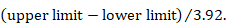
For 90% confidence intervals 3.92 should be replaced by 3.29, and for 99% confidence intervals it should be replaced by 5.15. Specific considerations are required for continuous outcome data when extracting mean differences. This is because confidence intervals should have been computed using t distributions, especially when the sample sizes are small: see Section 6.5.2.3 for details.
Where exact P values are quoted alongside estimates of intervention effect, it is possible to derive SEs. While all tests of statistical significance produce P values, different tests use different mathematical approaches. The method here assumes P values have been obtained through a particularly simple approach of dividing the effect estimate by its SE and comparing the result (denoted Z) with a standard normal distribution (statisticians often refer to this as a Wald test).
The first step is to obtain the Z value corresponding to the reported P value from a table of the standard normal distribution. A SE may then be calculated as
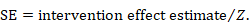
As an example, suppose a conference abstract presents an estimate of a risk difference of 0.03 (P = 0.008). The Z value that corresponds to a P value of 0.008 is Z = 2.652. This can be obtained from a table of the standard normal distribution or a computer program (for example, by entering =abs(normsinv(0.008/2)) into any cell in a Microsoft Excel spreadsheet). The SE of the risk difference is obtained by dividing the risk difference (0.03) by the Z value (2.652), which gives 0.011.
Where significance tests have used other mathematical approaches, the estimated SEs may not coincide exactly with the true SEs. For P values that are obtained from t-tests for continuous outcome data, refer instead to Section 6.5.2.3.
6.3.2 Obtaining standard errors from confidence intervals and P values: ratio measures
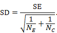
The process of obtaining SE for ratio measures is similar to that for absolute measures, but with an additional first step. Analyses of ratio measures are performed on the natural log scale (see Section 6.1.2.1). For a ratio measure, such as a risk ratio, odds ratio or hazard ratio (which we denote generically as RR here), first calculate


Then the formulae in Section 6.3.1 can be used. Note that the SE refers to the log of the ratio measure. When using the generic inverse variance method in RevMan, the data should be entered on the natural log scale, that is as lnRR and the SE of lnRR, as calculated here (see Chapter 10, Section 10.3).
6.4 Dichotomous outcome data
6.4.1 Effect measures for dichotomous outcomes
Dichotomous (binary) outcome data arise when the outcome for every participant is one of two possibilities, for example, dead or alive, or clinical improvement or no clinical improvement. This section considers the possible summary statistics to use when the outcome of interest has such a binary form. The most commonly encountered effect measures used in randomized trials with dichotomous data are:
- the risk ratio (RR; also called the relative risk);
- the odds ratio (OR);
- the risk difference (RD; also called the absolute risk reduction); and
- the number needed to treat for an additional beneficial or harmful outcome (NNT).
Details of the calculations of the first three of these measures are given in Box 6.4.a. Numbers needed to treat are discussed in detail in Chapter 15, Section 15.4, as they are primarily used for the communication and interpretation of results.
Methods for meta-analysis of dichotomous outcome data are covered in Chapter 10, Section 10.4.
Aside: as events of interest may be desirable rather than undesirable, it would be preferable to use a more neutral term than risk (such as probability), but for the sake of convention we use the terms risk ratio and risk difference throughout. We also use the term ‘risk ratio’ in preference to ‘relative risk’ for consistency with other terminology. The two are interchangeable and both conveniently abbreviate to ‘RR’. Note also that we have been careful with the use of the words ‘risk’ and ‘rates’. These words are often treated synonymously. However, we have tried to reserve use of the word ‘rate’ for the data type ‘counts and rates’ where it describes the frequency of events in a measured period of time.
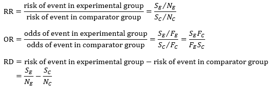
Box 6.4.a Calculation of risk ratio (RR), odds ratio (OR) and risk difference (RD) from a 2×2 table
|
The results of a two-group randomized trial with a dichotomous outcome can be displayed as a 2✕2 table:
where SE, SC, FE and FC are the numbers of participants with each outcome (‘S’ or ‘F’) in each group (‘E’ or ‘C’). The following summary statistics can be calculated: |
6.4.1.1 Risk and odds
In general conversation the terms ‘risk’ and ‘odds’ are used interchangeably (and also with the terms ‘chance’, ‘probability’ and ‘likelihood’) as if they describe the same quantity. In statistics, however, risk and odds have particular meanings and are calculated in different ways. When the difference between them is ignored, the results of a systematic review may be misinterpreted.
Risk is the concept more familiar to health professionals and the general public. Risk describes the probability with which a health outcome will occur. In research, risk is commonly expressed as a decimal number between 0 and 1, although it is occasionally converted into a percentage. In ‘Summary of findings’ tables in Cochrane Reviews, it is often expressed as a number of individuals per 1000 (see Chapter 14, Section 14.1.4). It is simple to grasp the relationship between a risk and the likely occurrence of events: in a sample of 100 people the number of events observed will on average be the risk multiplied by 100. For example, when the risk is 0.1, about 10 people out of every 100 will have the event; when the risk is 0.5, about 50 people out of every 100 will have the event. In a sample of 1000 people, these numbers are 100 and 500 respectively.
Odds is a concept that may be more familiar to gamblers. The ‘odds’ refers to the ratio of the probability that a particular event will occur to the probability that it will not occur, and can be any number between zero and infinity. In gambling, the odds describes the ratio of the size of the potential winnings to the gambling stake; in health care it is the ratio of the number of people with the event to the number without. It is commonly expressed as a ratio of two integers. For example, an odds of 0.01 is often written as 1:100, odds of 0.33 as 1:3, and odds of 3 as 3:1. Odds can be converted to risks, and risks to odds, using the formulae:
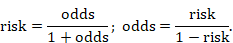
The interpretation of odds is more complicated than for a risk. The simplest way to ensure that the interpretation is correct is first to convert the odds into a risk. For example, when the odds are 1:10, or 0.1, one person will have the event for every 10 who do not, and, using the formula, the risk of the event is 0.1/(1+0.1)=0.091. In a sample of 100, about 9 individuals will have the event and 91 will not. When the odds are equal to 1, one person will have the event for every person who does not, so in a sample of 100, 100✕1/(1+1)=50 will have the event and 50 will not.
The difference between odds and risk is small when the event is rare (as illustrated in the example above where a risk of 0.091 was seen to be similar to an odds of 0.1). When events are common, as is often the case in clinical trials, the differences between odds and risks are large. For example, a risk of 0.5 is equivalent to an odds of 1; and a risk of 0.95 is equivalent to odds of 19.
Effect measures for randomized trials with dichotomous outcomes involve comparing either risks or odds from two intervention groups. To compare them we can look at their ratio (risk ratio or odds ratio) or the difference in risk (risk difference).
6.4.1.2 Measures of relative effect: the risk ratio and odds ratio
Measures of relative effect express the expected outcome in one group relative to that in the other. The risk ratio (RR, or relative risk) is the ratio of the risk of an event in the two groups, whereas the odds ratio (OR) is the ratio of the odds of an event (see Box 6.4.a). For both measures a value of 1 indicates that the estimated effects are the same for both interventions.
Neither the risk ratio nor the odds ratio can be calculated for a study if there are no events in the comparator group. This is because, as can be seen from the formulae in Box 6.4.a, we would be trying to divide by zero. The odds ratio also cannot be calculated if everybody in the intervention group experiences an event. In these situations, and others where SEs cannot be computed, it is customary to add ½ to each cell of the 2✕2 table (for example, RevMan automatically makes this correction when necessary). In the case where no events (or all events) are observed in both groups the study provides no information about relative probability of the event and is omitted from the meta-analysis. This is entirely appropriate. Zeros arise particularly when the event of interest is rare, such as unintended adverse outcomes. For further discussion of choice of effect measures for such sparse data (often with lots of zeros) see Chapter 10, Section 10.4.4.
Risk ratios describe the multiplication of the risk that occurs with use of the experimental intervention. For example, a risk ratio of 3 for an intervention implies that events with intervention are three times more likely than events without intervention. Alternatively we can say that intervention increases the risk of events by 100×(RR–1)%=200%. Similarly, a risk ratio of 0.25 is interpreted as the probability of an event with intervention being one-quarter of that without intervention. This may be expressed alternatively by saying that intervention decreases the risk of events by 100×(1–RR)%=75%. This is known as the relative risk reduction (see also Chapter 15, Section 15.4.1). The interpretation of the clinical importance of a given risk ratio cannot be made without knowledge of the typical risk of events without intervention: a risk ratio of 0.75 could correspond to a clinically important reduction in events from 80% to 60%, or a small, less clinically important reduction from 4% to 3%. What constitutes clinically important will depend on the outcome and the values and preferences of the person or population.
The numerical value of the observed risk ratio must always be between 0 and 1/CGR, where CGR (abbreviation of ‘comparator group risk’, sometimes referred to as the control group risk or the control event rate) is the observed risk of the event in the comparator group expressed as a number between 0 and 1. This means that for common events large values of risk ratio are impossible. For example, when the observed risk of events in the comparator group is 0.66 (or 66%) then the observed risk ratio cannot exceed 1.5. This boundary applies only for increases in risk, and can cause problems when the results of an analysis are extrapolated to a different population in which the comparator group risks are above those observed in the study.
Odds ratios, like odds, are more difficult to interpret (Sinclair and Bracken 1994, Sackett et al 1996). Odds ratios describe the multiplication of the odds of the outcome that occur with use of the intervention. To understand what an odds ratio means in terms of changes in numbers of events it is simplest to convert it first into a risk ratio, and then interpret the risk ratio in the context of a typical comparator group risk, as outlined here. The formula for converting an odds ratio to a risk ratio is provided in Chapter 15, Section 15.4.4. Sometimes it may be sensible to calculate the RR for more than one assumed comparator group risk.
6.4.1.3 Warning: OR and RR are not the same
Since risk and odds are different when events are common, the risk ratio and the odds ratio also differ when events are common. This non-equivalence does not indicate that either is wrong: both are entirely valid ways of describing an intervention effect. Problems may arise, however, if the odds ratio is misinterpreted as a risk ratio. For interventions that increase the chances of events, the odds ratio will be larger than the risk ratio, so the misinterpretation will tend to overestimate the intervention effect, especially when events are common (with, say, risks of events more than 20%). For interventions that reduce the chances of events, the odds ratio will be smaller than the risk ratio, so that, again, misinterpretation overestimates the effect of the intervention. This error in interpretation is unfortunately quite common in published reports of individual studies and systematic reviews.
6.4.1.4 Measure of absolute effect: the risk difference
The risk difference is the difference between the observed risks (proportions of individuals with the outcome of interest) in the two groups (see Box 6.4.a). The risk difference can be calculated for any study, even when there are no events in either group. The risk difference is straightforward to interpret: it describes the difference in the observed risk of events between experimental and comparator interventions; for an individual it describes the estimated difference in the probability of experiencing the event. However, the clinical importance of a risk difference may depend on the underlying risk of events in the population. For example, a risk difference of 0.02 (or 2%) may represent a small, clinically insignificant change from a risk of 58% to 60% or a proportionally much larger and potentially important change from 1% to 3%. Although the risk difference provides more directly relevant information than relative measures (Laupacis et al 1988, Sackett et al 1997), it is still important to be aware of the underlying risk of events, and consequences of the events, when interpreting a risk difference. Absolute measures, such as the risk difference, are particularly useful when considering trade-offs between likely benefits and likely harms of an intervention.
The risk difference is naturally constrained (like the risk ratio), which may create difficulties when applying results to other patient groups and settings. For example, if a study or meta-analysis estimates a risk difference of –0.1 (or –10%), then for a group with an initial risk of, say, 7% the outcome will have an impossible estimated negative probability of –3%. Similar scenarios for increases in risk occur at the other end of the scale. Such problems can arise only when the results are applied to populations with different risks from those observed in the studies.
The number needed to treat is obtained from the risk difference. Although it is often used to summarize results of clinical trials, NNTs cannot be combined in a meta-analysis (see Chapter 10, Section 10.4.3). However, odds ratios, risk ratios and risk differences may be usefully converted to NNTs and used when interpreting the results of a meta-analysis as discussed in Chapter 15, Section 15.4.
6.4.1.5 What is the event?
In the context of dichotomous outcomes, healthcare interventions are intended either to reduce the risk of occurrence of an adverse outcome or increase the chance of a good outcome. It is common to use the term ‘event’ to describe whatever the outcome or state of interest is in the analysis of dichotomous data. For example, when participants have particular symptoms at the start of the study the event of interest is usually recovery or cure. If participants are well or, alternatively, at risk of some adverse outcome at the beginning of the study, then the event is the onset of disease or occurrence of the adverse outcome.
It is possible to switch events and non-events and consider instead the proportion of patients not recovering or not experiencing the event. For meta-analyses using risk differences or odds ratios the impact of this switch is of no great consequence: the switch simply changes the sign of a risk difference, indicating an identical effect size in the opposite direction, whilst for odds ratios the new odds ratio is the reciprocal (1/x) of the original odds ratio.
In contrast, switching the outcome can make a substantial difference for risk ratios, affecting the effect estimate, its statistical significance, and the consistency of intervention effects across studies. This is because the precision of a risk ratio estimate differs markedly between those situations where risks are low and those where risks are high. In a meta-analysis, the effect of this reversal cannot be predicted easily. The identification, before data analysis, of which risk ratio is more likely to be the most relevant summary statistic is therefore important. It is often convenient to choose to focus on the event that represents a change in state. For example, in treatment studies where everyone starts in an adverse state and the intention is to ‘cure’ this, it may be more natural to focus on ‘cure’ as the event. Alternatively, in prevention studies where everyone starts in a ‘healthy’ state and the intention is to prevent an adverse event, it may be more natural to focus on ‘adverse event’ as the event. A general rule of thumb is to focus on the less common state as the event of interest. This reduces the problems associated with extrapolation (see Section 6.4.1.2) and may lead to less heterogeneity across studies. Where interventions aim to reduce the incidence of an adverse event, there is empirical evidence that risk ratios of the adverse event are more consistent than risk ratios of the non-event (Deeks 2002).
6.4.2 Data extraction for dichotomous outcomes
To calculate summary statistics and include the result in a meta-analysis, the only data required for a dichotomous outcome are the numbers of participants in each of the intervention groups who did and did not experience the outcome of interest (the numbers needed to fill in a standard 2×2 table, as in Box 6.4.a). In RevMan, these can be entered as the numbers with the outcome and the total sample sizes for the two groups. Although in theory this is equivalent to collecting the total numbers and the numbers experiencing the outcome, it is not always clear whether the reported total numbers are the whole sample size or only those for whom the outcome was measured or observed. Collecting the numbers of actual observations is preferable, as it avoids assumptions about any participants for whom the outcome was not measured. Occasionally the numbers of participants who experienced the event must be derived from percentages (although it is not always clear which denominator to use, because rounded percentages may be compatible with more than one numerator).
Sometimes the numbers of participants and numbers of events are not available, but an effect estimate such as an odds ratio or risk ratio may be reported. Such data may be included in meta-analyses (using the generic inverse variance method) only when they are accompanied by measures of uncertainty such as a SE, 95% confidence interval or an exact P value (see Section 6.3).
6.5 Continuous outcome data
6.5.1 Effect measures for continuous outcomes
The term ‘continuous’ in statistics conventionally refers to a variable that can take any value in a specified range. When dealing with numerical data, this means that a number may be measured and reported to an arbitrary number of decimal places. Examples of truly continuous data are weight, area and volume. In practice, we can use the same statistical methods for other types of data, most commonly measurement scales and counts of large numbers of events (see Section 6.6.1).
A common feature of continuous data is that a measurement used to assess the outcome of each participant is also measured at baseline, that is, before interventions are administered. This gives rise to the possibility of computing effects based on change from baseline (also called a change score). When effect measures are based on change from baseline, a single measurement is created for each participant, obtained either by subtracting the post-intervention measurement from the baseline measurement or by subtracting the baseline measurement from the post-intervention measurement. Analyses then proceed as for any other type of continuous outcome variable.
Two summary statistics are commonly used for meta-analysis of continuous data: the mean difference and the standardized mean difference. These can be calculated whether the data from each individual are post-intervention measurements or change-from-baseline measures. It is also possible to measure effects by taking ratios of means, or to use other alternatives.
Sometimes review authors may consider dichotomizing continuous outcome measures so that the result of the trial can be expressed as an odds ratio, risk ratio or risk difference. This might be done either to improve interpretation of the results (see Chapter 15, Section 15.5), or because the majority of the studies present results after dichotomizing a continuous measure. Results reported as means and SDs can, under some assumptions, be converted to risks (Anzures-Cabrera et al 2011). Typically a normal distribution is assumed for the outcome variable within each intervention group.
Methods for meta-analysis of continuous outcome data are covered in Chapter 10, Section 10.5.
6.5.1.1 The mean difference (or difference in means)
The mean difference (MD, or more correctly, ‘difference in means’) is a standard statistic that measures the absolute difference between the mean value in two groups of a randomized trial. It estimates the amount by which the experimental intervention changes the outcome on average compared with the comparator intervention. It can be used as a summary statistic in meta-analysis when outcome measurements in all studies are made on the same scale.
Aside: analyses based on this effect measure were historically termed ‘weighted mean difference’ (WMD) analyses in the Cochrane Database of Systematic Reviews. This name is potentially confusing: although the meta-analysis computes a weighted average of these differences in means, no weighting is involved in calculation of a statistical summary of a single study. Furthermore, all meta-analyses involve a weighted combination of estimates, yet we do not use the word ‘weighted’ when referring to other methods.
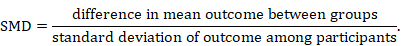
6.5.1.2 The standardized mean difference
The standardized mean difference (SMD) is used as a summary statistic in meta-analysis when the studies all assess the same outcome, but measure it in a variety of ways (for example, all studies measure depression but they use different psychometric scales). In this circumstance it is necessary to standardize the results of the studies to a uniform scale before they can be combined. The SMD expresses the size of the intervention effect in each study relative to the between-participant variability in outcome measurements observed in that study. (Again in reality the intervention effect is a difference in means and not a mean of differences.)
Thus, studies for which the difference in means is the same proportion of the standard deviation (SD) will have the same SMD, regardless of the actual scales used to make the measurements.
However, the method assumes that the differences in SDs among studies reflect differences in measurement scales and not real differences in variability among study populations. If in two trials the true effect (as measured by the difference in means) is identical, but the SDs are different, then the SMDs will be different. This may be problematic in some circumstances where real differences in variability between the participants in different studies are expected. For example, where early explanatory trials are combined with later pragmatic trials in the same review, pragmatic trials may include a wider range of participants and may consequently have higher SDs. The overall intervention effect can also be difficult to interpret as it is reported in units of SD rather than in units of any of the measurement scales used in the review, but several options are available to aid interpretation (see Chapter 15, Section 15.6).
The term ‘effect size’ is frequently used in the social sciences, particularly in the context of meta-analysis. Effect sizes typically, though not always, refer to versions of the SMD. It is recommended that the term ‘SMD’ be used in Cochrane Reviews in preference to ‘effect size’ to avoid confusion with the more general plain language use of the latter term as a synonym for ‘intervention effect’ or ‘effect estimate’.
It should be noted that the SMD method does not correct for differences in the direction of the scale. If some scales increase with disease severity (for example, a higher score indicates more severe depression) whilst others decrease (a higher score indicates less severe depression), it is essential to multiply the mean values from one set of studies by –1 (or alternatively to subtract the mean from the maximum possible value for the scale) to ensure that all the scales point in the same direction, before standardization (see MECIR Box 6.5.a). Any such adjustment should be described in the statistical methods section of the review. The SD does not need to be modified.
MECIR Box 6.5.a Relevant expectations for conduct of intervention reviews
|
C61: Combining different scales (Mandatory) |
|
|
If studies are combined with different scales, ensure that higher scores for continuous outcomes all have the same meaning for any particular outcome; explain the direction of interpretation; and report when directions are reversed. |
Sometimes scales have higher scores that reflect a ‘better’ outcome and sometimes lower scores reflect ‘better’ outcome. Meaningless (and misleading) results arise when effect estimates with opposite clinical meanings are combined. |
Different variations on the SMD are available depending on exactly what choice of SD is chosen for the denominator. The particular definition of SMD used in Cochrane Reviews is the effect size known in social science as Hedges’ (adjusted) g. This uses a pooled SD in the denominator, which is an estimate of the SD based on outcome data from both intervention groups, assuming that the SDs in the two groups are similar. In contrast, Glass’ delta (Δ) uses only the SD from the comparator group, on the basis that if the experimental intervention affects between-person variation, then such an impact of the intervention should not influence the effect estimate.
To overcome problems associated with estimating SDs within small studies, and with real differences across studies in between-person variability, it may sometimes be desirable to standardize using an external estimate of SD. External estimates might be derived, for example, from a cross-sectional analysis of many individuals assessed using the same continuous outcome measure (the sample of individuals might be derived from a large cohort study). Typically the external estimate would be assumed to be known without error, which is likely to be reasonable if it is based on a large number of individuals. Under this assumption, the statistical methods used for MDs would be used, with both the MD and its SE divided by the externally derived SD.
6.5.1.3 The ratio of means
The ratio of means (RoM) is a less commonly used statistic that measures the relative difference between the mean value in two groups of a randomized trial (Friedrich et al 2008). It estimates the amount by which the average value of the outcome is multiplied for participants on the experimental intervention compared with the comparator intervention. For example, a RoM of 2 for an intervention implies that the mean score in the participants receiving the experimental intervention is on average twice as high as that of the group without intervention. It can be used as a summary statistic in meta-analysis when outcome measurements can only be positive. Thus it is suitable for single (post-intervention) assessments but not for change-from-baseline measures (which can be negative).
An advantage of the RoM is that it can be used in meta-analysis to combine results from studies that used different measurement scales. However, it is important that these different scales have comparable lower limits. For example, a RoM might meaningfully be used to combine results from a study using a scale ranging from 0 to 10 with results from a study ranging from 1 to 50. However, it is unlikely to be reasonable to combine RoM results from a study using a scale ranging from 0 to 10 with RoM results from a study using a scale ranging from 20 to 30: it is not possible to obtain RoM values outside of the range 0.67 to 1.5 in the latter study, whereas such values are readily obtained in the former study. RoM is not a suitable effect measure for the latter study.
The RoM might be a particularly suitable choice of effect measure when the outcome is a physical measurement that can only take positive values, but when different studies use different measurement approaches that cannot readily be converted from one to another. For example, it was used in a meta-analysis where studies assessed urine output using some measures that did, and some measures that did not, adjust for body weight (Friedrich et al 2005).
6.5.1.4 Other effect measures for continuous outcome data
Other effect measures for continuous outcome data include the following:
- Standardized difference in terms of the minimal important differences (MID) on each scale. This expresses the MD as a proportion of the amount of change on a scale that would be considered clinically meaningful (Johnston et al 2010).
- Prevented fraction. This expresses the MD in change scores in relation to the comparator group mean change. Thus it describes how much change in the comparator group might have been prevented by the experimental intervention. It has commonly been used in dentistry (Dubey et al 1965).
- Difference in percentage change from baseline. This is a version of the MD in which each intervention group is summarized by the mean change divided by the mean baseline level, thus expressing it as a percentage. The measure has often been used, for example, for outcomes such as cholesterol level, blood pressure and glaucoma. Care is needed to ensure that the SE correctly accounts for correlation between baseline and post-intervention values (Vickers 2001).
- Direct mapping from one scale to another. If conversion factors are available that map one scale to another (e.g. pounds to kilograms) then these should be used. Methods are also available that allow these conversion factors to be estimated (Ades et al 2015).
6.5.2 Data extraction for continuous outcomes
To perform a meta-analysis of continuous data using MDs, SMDs or ratios of means, review authors should seek:
- the mean value of the outcome measurements in each intervention group;
- the standard deviation of the outcome measurements in each intervention group; and
- the number of participants for whom the outcome was measured in each intervention group.
Due to poor and variable reporting it may be difficult or impossible to obtain these numbers from the data summaries presented. Studies vary in the statistics they use to summarize the average (sometimes using medians rather than means) and variation (sometimes using SEs, confidence intervals, interquartile ranges and ranges rather than SDs). They also vary in the scale chosen to analyse the data (e.g. post-intervention measurements versus change from baseline; raw scale versus logarithmic scale).
A particularly misleading error is to misinterpret a SE as a SD. Unfortunately, it is not always clear which is being reported and some intelligent reasoning, and comparison with other studies, may be required. SDs and SEs are occasionally confused in the reports of studies, and the terminology is used inconsistently.
When needed, missing information and clarification about the statistics presented should always be sought from the authors. However, for several measures of variation there is an approximate or direct algebraic relationship with the SD, so it may be possible to obtain the required statistic even when it is not published in a paper, as explained in Sections 6.5.2.1 to 6.5.2.6. More details and examples are available elsewhere (Deeks 1997a, Deeks 1997b). Section 6.5.2.7 discusses options whenever SDs remain missing after attempts to obtain them.
Sometimes the numbers of participants, means and SDs are not available, but an effect estimate such as a MD or SMD has been reported. Such data may be included in meta-analyses using the generic inverse variance method only when they are accompanied by measures of uncertainty such as a SE, 95% confidence interval or an exact P value. A suitable SE from a confidence interval for a MD should be obtained using the early steps of the process described in Section 6.5.2.3. For SMDs, see Section 6.3.
6.5.2.1 Extracting post-intervention versus change from baseline data
Commonly, studies in a review will have reported a mixture of changes from baseline and post-intervention values (i.e. values at various follow-up time points, including ‘final value’). Some studies will report both; others will report only change scores or only post-intervention values. As explained in Chapter 10, Section 10.5.2, both post-intervention values and change scores can sometimes be combined in the same analysis so this is not necessarily a problem. Authors may wish to extract data on both change from baseline and post-intervention outcomes if the required means and SDs are available (see Section 6.5.2.7 for cases where the applicable SDs are not available). The choice of measure reported in the studies may be associated with the direction and magnitude of results. Review authors should seek evidence of whether such selective reporting may be the case in one or more studies (see Chapter 8, Section 8.7).
A final problem with extracting information on change from baseline measures is that often baseline and post-intervention measurements may have been reported for different numbers of participants due to missed visits and study withdrawals. It may be difficult to identify the subset of participants who report both baseline and post-intervention measurements for whom change scores can be computed.
6.5.2.2 Obtaining standard deviations from standard errors and confidence intervals for group means
A standard deviation can be obtained from the SE of a mean by multiplying by the square root of the sample size:
 .
.
When making this transformation, the SE must be calculated from within a single intervention group, and must not be the SE of the mean difference between two intervention groups.
The confidence interval for a mean can also be used to calculate the SD. Again, the following applies to the confidence interval for a mean value calculated within an intervention group and not for estimates of differences between interventions (for these, see Section 6.5.2.3). Most reported confidence intervals are 95% confidence intervals. If the sample size is large (say larger than 100 in each group), the 95% confidence interval is 3.92 SE wide (3.92=2✕1.96). The SD for each group is obtained by dividing the width of the confidence interval by 3.92, and then multiplying by the square root of the sample size in that group:
 .
.
For 90% confidence intervals, 3.92 should be replaced by 3.29, and for 99% confidence intervals it should be replaced by 5.15.
If the sample size is small (say fewer than 60 participants in each group) then confidence intervals should have been calculated using a value from a t distribution. The numbers 3.92, 3.29 and 5.15 are replaced with slightly larger numbers specific to the t distribution, which can be obtained from tables of the t distribution with degrees of freedom equal to the group sample size minus 1. Relevant details of the t distribution are available as appendices of many statistical textbooks or from standard computer spreadsheet packages. For example the t statistic for a 95% confidence interval from a sample size of 25 can be obtained by typing =tinv(1-0.95,25-1) in a cell in a Microsoft Excel spreadsheet (the result is 2.0639). The divisor, 3.92, in the formula above would be replaced by 2✕2.0639=4.128.
For moderate sample sizes (say between 60 and 100 in each group), either a t distribution or a standard normal distribution may have been used. Review authors should look for evidence of which one, and use a t distribution when in doubt.
As an example, consider data presented as follows:
|
Group |
Sample size |
Mean |
95% CI |
|
Experimental intervention |
25 |
32.1 |
(30.0, 34.2) |
|
Comparator intervention |
22 |
28.3 |
(26.5, 30.1) |
The confidence intervals should have been based on t distributions with 24 and 21 degrees of freedom, respectively. The divisor for the experimental intervention group is 4.128, from above. The SD for this group is √25✕(34.2–30.0)/4.128=5.09. Calculations for the comparator group are performed in a similar way.
It is important to check that the confidence interval is symmetrical about the mean (the distance between the lower limit and the mean is the same as the distance between the mean and the upper limit). If this is not the case, the confidence interval may have been calculated on transformed values (see Section 6.5.2.4).
6.5.2.3 Obtaining standard deviations from standard errors, confidence intervals, t statistics and P values for differences in means
Standard deviations can be obtained from a SE, confidence interval, t statistic or P value that relates to a difference between means in two groups (i.e. the MD). The MD is required in the calculations from the t statistic or the P value. An assumption that the SDs of outcome measurements are the same in both groups is required in all cases. The same SD is then used for both intervention groups. We describe first how a t statistic can be obtained from a P value, then how a SE can be obtained from a t statistic or a confidence interval, and finally how a SD is obtained from the SE. Review authors may select the appropriate steps in this process according to what results are available to them. Related methods can be used to derive SDs from certain F statistics, since taking the square root of an F statistic may produce the same t statistic. Care often is required to ensure that an appropriate F statistic is used. Advice from a knowledgeable statistician is recommended.
(1) From P value to t statistic
Where actual P values obtained from t-tests are quoted, the corresponding t statistic may be obtained from a table of the t distribution. The degrees of freedom are given by NE+NC–2, where NE and NC are the sample sizes in the experimental and comparator groups. We will illustrate with an example. Consider a trial of an experimental intervention (NE=25) versus a comparator intervention (NC=22), where the MD=3.8. The P value for the comparison was P=0.008, obtained using a two-sample t-test.
The t statistic that corresponds with a P value of 0.008 and 25+22–2=45 degrees of freedom is t=2.78. This can be obtained from a table of the t distribution with 45 degrees of freedom or a computer (for example, by entering =tinv(0.008, 45) into any cell in a Microsoft Excel spreadsheet).
Difficulties are encountered when levels of significance are reported (such as P<0.05 or even P=NS (‘not significant’, which usually implies P>0.05) rather than exact P values. A conservative approach would be to take the P value at the upper limit (e.g. for P<0.05 take P=0.05, for P<0.01 take P=0.01 and for P<0.001 take P=0.001). However, this is not a solution for results that are reported as P=NS, or P>0.05 (see Section 6.5.2.7).
(2) From t statistic to standard error
The t statistic is the ratio of the MD to the SE of the MD. The SE of the MD can therefore be obtained by dividing it by the t statistic:

where  denotes ‘the absolute value of X’. In the example, where MD=3.8 and t=2.78, the SE of the MD is obtained by dividing 3.8 by 2.78, which gives 1.37.
(3) From confidence interval to standard error
If a 95% confidence interval is available for the MD, then the same SE can be calculated as:
 ,
,
as long as the trial is large. For 90% confidence intervals divide by 3.29 rather than 3.92; for 99% confidence intervals divide by 5.15. If the sample size is small (say fewer than 60 participants in each group) then confidence intervals should have been calculated using a t distribution. The numbers 3.92, 3.29 and 5.15 are replaced with larger numbers specific to both the t distribution and the sample size, and can be obtained from tables of the t distribution with degrees of freedom equal to NE+NC–2, where NE and NC are the sample sizes in the two groups. Relevant details of the t distribution are available as appendices of many statistical textbooks or from standard computer spreadsheet packages. For example, the t statistic for a 95% confidence interval from a comparison of a sample size of 25 with a sample size of 22 can be obtained by typing =tinv(1-0.95,25+22-2) in a cell in a Microsoft Excel spreadsheet.
(4) From standard error to standard deviation
The within-group SD can be obtained from the SE of the MD using the following formula:
In the example,
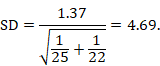
Note that this SD is the average of the SDs of the experimental and comparator arms, and should be entered into RevMan twice (once for each intervention group).
6.5.2.4 Transformations and skewed data
Studies may present summary statistics calculated after a transformation has been applied to the raw data. For example, means and SDs of logarithmic values may be available (or, equivalently, a geometric mean and its confidence interval). Such results should be collected, as they may be included in meta-analyses, or – with certain assumptions – may be transformed back to the raw scale (Higgins et al 2008).
For example, a trial reported meningococcal antibody responses 12 months after vaccination with meningitis C vaccine and a control vaccine (MacLennan et al 2000), as geometric mean titres of 24 and 4.2 with 95% confidence intervals of 17 to 34 and 3.9 to 4.6, respectively. These summaries were obtained by finding the means and confidence intervals of the natural logs of the antibody responses (for vaccine 3.18 (95% CI 2.83 to 3.53), and control 1.44 (1.36 to 1.53)), and taking their exponentials (anti-logs). A meta-analysis may be performed on the scale of these natural log antibody responses, rather than the geometric means. SDs of the log-transformed data may be derived from the latter pair of confidence intervals using methods described in Section 6.5.2.1. For further discussion of meta-analysis with skewed data, see Chapter 10, Section 10.5.3.
6.5.2.5 Interquartile ranges
Interquartile ranges describe where the central 50% of participants’ outcomes lie. When sample sizes are large and the distribution of the outcome is similar to the normal distribution, the width of the interquartile range will be approximately 1.35 SDs. In other situations, and especially when the outcome’s distribution is skewed, it is not possible to estimate a SD from an interquartile range. Note that the use of interquartile ranges rather than SDs often can indicate that the outcome’s distribution is skewed. Wan and colleagues provided a sample size-dependent extension to the formula for approximating the SD using the interquartile range (Wan et al 2014).
6.5.2.6 Ranges
Ranges are very unstable and, unlike other measures of variation, increase when the sample size increases. They describe the extremes of observed outcomes rather than the average variation. One common approach has been to make use of the fact that, with normally distributed data, 95% of values will lie within 2✕SD either side of the mean. The SD may therefore be estimated to be approximately one-quarter of the typical range of data values. This method is not robust and we recommend that it not be used. Walter and Yao based an imputation method on the minimum and maximum observed values. Their enhancement of the “range’ method provided a lookup table, according to sample size, of conversion factors from range to SD (Walter and Yao 2007). Alternative methods have been proposed to estimate SDs from ranges and quantiles (Hozo et al 2005, Wan et al 2014, Bland 2015), although to our knowledge these have not been evaluated using empirical data. As a general rule, we recommend that ranges should not be used to estimate SDs.
6.5.2.7 No information on variability
Missing SDs are a common feature of meta-analyses of continuous outcome data. When none of the above methods allow calculation of the SDs from the trial report (and the information is not available from the trialists) then a review author may be forced to impute (‘fill in’) the missing data if they are not to exclude the study from the meta-analysis.
The simplest imputation is to borrow the SD from one or more other studies. Furukawa and colleagues found that imputing SDs either from other studies in the same meta-analysis, or from studies in another meta-analysis, yielded approximately correct results in two case studies (Furukawa et al 2006). If several candidate SDs are available, review authors should decide whether to use their average, the highest, a ‘reasonably high’ value, or some other strategy. For meta-analyses of MDs, choosing a higher SD down-weights a study and yields a wider confidence interval. However, for SMD meta-analyses, choosing a higher SD will bias the result towards a lack of effect. More complicated alternatives are available for making use of multiple candidate SDs. For example, Marinho and colleagues implemented a linear regression of log(SD) on log(mean), because of a strong linear relationship between the two (Marinho et al 2003).
All imputation techniques involve making assumptions about unknown statistics, and it is best to avoid using them wherever possible. If the majority of studies in a meta-analysis have missing SDs, these values should not be imputed. A narrative approach might then be needed for the synthesis (see Chapter 12). However, imputation may be reasonable for a small proportion of studies comprising a small proportion of the data if it enables them to be combined with other studies for which full data are available. Sensitivity analyses should be used to assess the impact of changing the assumptions made.
6.5.2.8 Imputing standard deviations for changes from baseline
A special case of missing SDs is for changes from baseline measurements. Often, only the following information is available:
|
Baseline |
Final |
Change |
|
|
Experimental intervention (sample size) |
mean, SD |
mean, SD |
mean |
|
Comparator intervention (sample size) |
mean, SD |
mean, SD |
mean |
Note that the mean change in each group can be obtained by subtracting the post-intervention mean from the baseline mean even if it has not been presented explicitly. However, the information in this table does not allow us to calculate the SD of the changes. We cannot know whether the changes were very consistent or very variable across individuals. Some other information in a paper may help us determine the SD of the changes.
When there is not enough information available in a paper to calculate the SDs for the changes, they can be imputed, for example, by using change-from-baseline SDs for the same outcome measure from other studies in the review. However, the appropriateness of using a SD from another study relies on whether the studies used the same measurement scale, had the same degree of measurement error, had the same time interval between baseline and post-intervention measurement, and in a similar population.
When statistical analyses comparing the changes themselves are presented (e.g. confidence intervals, SEs, t statistics, P values, F statistics) then the techniques described in Section 6.5.2.3 may be used. Also note that an alternative to these methods is simply to use a comparison of post-intervention measurements, which in a randomized trial in theory estimates the same quantity as the comparison of changes from baseline.
The following alternative technique may be used for calculating or imputing missing SDs for changes from baseline (Follmann et al 1992, Abrams et al 2005). A typically unreported number known as the correlation coefficient describes how similar the baseline and post-intervention measurements were across participants. Here we describe (1) how to calculate the correlation coefficient from a study that is reported in considerable detail and (2) how to impute a change-from-baseline SD in another study, making use of a calculated or imputed correlation coefficient. Note that the methods in (2) are applicable both to correlation coefficients obtained using (1) and to correlation coefficients obtained in other ways (for example, by reasoned argument). Methods in (2) should be used sparingly because one can never be sure that an imputed correlation is appropriate. This is because correlations between baseline and post-intervention values usually will, for example, decrease with increasing time between baseline and post-intervention measurements, as well as depending on the outcomes, characteristics of the participants and intervention effects.
(1) Calculating a correlation coefficient from a study reported in considerable detail
Suppose a study presents means and SDs for change as well as for baseline and post-intervention (‘Final’) measurements, for example:
|
|
Baseline |
Final |
Change |
|
Experimental intervention (sample size 129) |
mean = 15.2 SD = 6.4 |
mean = 16.2 SD = 7.1 |
mean = 1.0 SD = 4.5 |
|
Comparator intervention (sample size 135) |
mean = 15.7 SD = 7.0 |
mean = 17.2 SD = 6.9 |
mean = 1.5 SD = 4.2 |
An analysis of change from baseline is available from this study, using only the data in the final column. We can use other data in this study to calculate two correlation coefficients, one for each intervention group. Let us use the following notation:
|
Baseline |
Final |
Change |
|
|
Experimental intervention (sample size |
|
|
|
|
Comparator intervention (sample size |
|
|
|
 )
) ,
, 
 ,
, 
 ,
, 
 )
) ,
, 
 ,
, 
 ,
, 
The correlation coefficient in the experimental group, CorrE, can be calculated as:
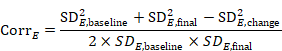
and similarly for the comparator intervention, to obtain CorrC. In the example, these turn out to be
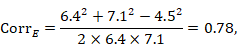
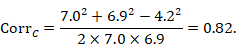
When either the baseline or post-intervention SD is unavailable, then it may be substituted by the other, providing it is reasonable to assume that the intervention does not alter the variability of the outcome measure. Assuming the correlation coefficients from the two intervention groups are reasonably similar to each other, a simple average can be taken as a reasonable measure of the similarity of baseline and final measurements across all individuals in the study (in the example, the average of 0.78 and 0.82 is 0.80). It is recommended that correlation coefficients be computed for many (if not all) studies in the meta-analysis and examined for consistency. If the correlation coefficients differ, then either the sample sizes are too small for reliable estimation, the intervention is affecting the variability in outcome measures, or the intervention effect depends on baseline level, and the use of average is best avoided. In addition, if a value less than 0.5 is obtained (correlation coefficients lie between –1 and 1), then there is little benefit in using change from baseline and an analysis of post-intervention measurements will be more precise.
(2) Imputing a change-from-baseline standard deviation using a correlation coefficient
Now consider a study for which the SD of changes from baseline is missing. When baseline and post-intervention SDs are known, we can impute the missing SD using an imputed value, Corr, for the correlation coefficient. The value Corr may be calculated from another study in the meta-analysis (using the method in (1)), imputed from elsewhere, or hypothesized based on reasoned argument. In all of these situations, a sensitivity analysis should be undertaken, trying different values of Corr, to determine whether the overall result of the analysis is robust to the use of imputed correlation coefficients.
To impute a SD of the change from baseline for the experimental intervention, use
 ,
,
and similarly for the comparator intervention. Again, if either of the SDs (at baseline and post-intervention) is unavailable, then one may be substituted by the other as long as it is reasonable to assume that the intervention does not alter the variability of the outcome measure.
As an example, consider the following data:
|
|
Baseline |
Final |
Change |
|
Experimental intervention (sample size 35) |
mean = 12.4 SD = 4.2 |
mean = 15.2 SD = 3.8 |
mean = 2.8 |
|
Comparator intervention (sample size 38) |
mean = 10.7 SD = 4.0 |
mean = 13.8 SD = 4.4 |
mean = 3.1 |
Using the correlation coefficient calculated in step 1 above of 0.80, we can impute the change-from-baseline SD in the comparator group as:

6.5.2.9 Missing means
Missing mean values sometimes occur for continuous outcome data. If a median is available instead, then this will be very similar to the mean when the distribution of the data is symmetrical, and so occasionally can be used directly in meta-analyses. However, means and medians can be very different from each other when the data are skewed, and medians often are reported because the data are skewed (see Chapter 10, Section 10.5.3). Nevertheless, Hozo and colleagues conclude that the median may often be a reasonable substitute for a mean (Hozo et al 2005).
Wan and colleagues proposed a formula for imputing a missing mean value based on the lower quartile, median and upper quartile summary statistics (Wan et al 2014). Bland derived an approximation for a missing mean using the sample size, the minimum and maximum values, the lower and upper quartile values, and the median (Bland 2015). Both of these approaches assume normally distributed outcomes but have been observed to perform well when analysing skewed outcomes; the same simulation study indicated that the Wan method had better properties (Weir et al 2018). Caveats about imputing values summarized in Section 6.5.2.7 should be observed.
6.5.2.10 Combining groups
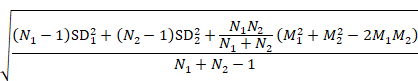
Sometimes it is desirable to combine two reported subgroups into a single group. For example, a study may report results separately for men and women in each of the intervention groups. The formulae in Table 6.5.a can be used to combine numbers into a single sample size, mean and SD for each intervention group (i.e. combining across men and women in each intervention group in this example). Note that the rather complex-looking formula for the SD produces the SD of outcome measurements as if the combined group had never been divided into two. This SD is different from the usual pooled SD that is used to compute a confidence interval for a MD or as the denominator in computing the SMD. This usual pooled SD provides a within-subgroup SD rather than an SD for the combined group, so provides an underestimate of the desired SD.
These formulae are also appropriate for use in studies that compared three or more interventions, two of which represent the same intervention category as defined for the purposes of the review. In that case, it may be appropriate to combine these two groups and consider them as a single intervention (see Chapter 23, Section 23.3). For example, ‘Group 1’ and ‘Group 2’ may refer to two slightly different variants of an intervention to which participants were randomized, such as different doses of the same drug.
When there are more than two groups to combine, the simplest strategy is to apply the above formula sequentially (i.e. combine Group 1 and Group 2 to create Group ‘1+2’, then combine Group ‘1+2’ and Group 3 to create Group ‘1+2+3’, and so on).
Table 6.5.a Formulae for combining summary statistics across two groups: Group 1 (with sample size = N1, mean = M1 and SD = SD1) and Group 2 (with sample size = N2, mean = M2 and SD = SD2)
|
Combined groups |
|
|
Sample size |
|
|
Mean |
|
|
SD |
|


6.6 Ordinal outcome data and measurement scales
6.6.1 Effect measures for ordinal outcomes and measurement scales
Ordinal outcome data arise when each participant is classified in a category and when the categories have a natural order. For example, a ‘trichotomous’ outcome such as the classification of disease severity into ‘mild’, ‘moderate’ or ‘severe’, is of ordinal type. As the number of categories increases, ordinal outcomes acquire properties similar to continuous outcomes, and probably will have been analysed as such in a randomized trial.
Measurement scales are one particular type of ordinal outcome frequently used to measure conditions that are difficult to quantify, such as behaviour, depression and cognitive abilities. Measurement scales typically involve a series of questions or tasks, each of which is scored and the scores then summed to yield a total ‘score’. If the items are not considered of equal importance a weighted sum may be used.
Methods are available for analysing ordinal outcome data that describe effects in terms of proportional odds ratios (Agresti 1996). Suppose that there are three categories, which are ordered in terms of desirability such that 1 is the best and 3 the worst. The data could be dichotomized in two ways: either category 1 constitutes a success and categories 2 and 3 a failure; or categories 1 and 2 constitute a success and category 3 a failure. A proportional odds model assumes that there is an equal odds ratio for both dichotomies of the data. Therefore, the odds ratio calculated from the proportional odds model can be interpreted as the odds of success on the experimental intervention relative to comparator, irrespective of how the ordered categories might be divided into success or failure. Methods (specifically polychotomous logistic regression models) are available for calculating study estimates of the log odds ratio and its SE.
Methods specific to ordinal data become unwieldy (and unnecessary) when the number of categories is large. In practice, longer ordinal scales acquire properties similar to continuous outcomes, and are often analysed as such, whilst shorter ordinal scales are often made into dichotomous data by combining adjacent categories together until only two remain. The latter is especially appropriate if an established, defensible cut-point is available. However, inappropriate choice of a cut-point can induce bias, particularly if it is chosen to maximize the difference between two intervention arms in a randomized trial.
Where ordinal scales are summarized using methods for dichotomous data, one of the two sets of grouped categories is defined as the event and intervention effects are described using risk ratios, odds ratios or risk differences (see Section 6.4.1). When ordinal scales are summarized using methods for continuous data, the mean score is calculated in each group and intervention effect is expressed as a MD or SMD, or possibly a RoM (see Section 6.5.1). Difficulties will be encountered if studies have summarized their results using medians (see Section 6.5.2.5). Methods for meta-analysis of ordinal outcome data are covered in Chapter 10, Section 10.7.
6.6.2 Data extraction for ordinal outcomes
The data to be extracted for ordinal outcomes depend on whether the ordinal scale will be dichotomized for analysis (see Section 6.4), treated as a continuous outcome (see Section 6.5.2) or analysed directly as ordinal data. This decision, in turn, will be influenced by the way in which study authors analysed and reported their data. It may be impossible to pre-specify whether data extraction will involve calculation of numbers of participants above and below a defined threshold, or mean values and SDs. In practice, it is wise to extract data in all forms in which they are given as it will not be clear which is the most common form until all studies have been reviewed. In some circumstances more than one form of analysis may justifiably be included in a review.
Where ordinal data are to be dichotomized and there are several options for selecting a cut-point (or the choice of cut-point is arbitrary) it is sensible to plan from the outset to investigate the impact of choice of cut-point in a sensitivity analysis (see Chapter 10, Section 10.14). To collect the data that would be used for each alternative dichotomization, it is necessary to record the numbers in each category of short ordinal scales to avoid having to extract data from a paper more than once. This approach of recording all categorizations is also sensible when studies used slightly different short ordinal scales and it is not clear whether there is a cut-point that is common across all the studies which can be used for dichotomization.
It is also necessary to record the numbers in each category of the ordinal scale for each intervention group when the proportional odds ratio method will be used (see Chapter 10, Section 10.7).
6.7 Count and rate data
6.7.1 Effect measures for counts and rates
Some types of event can happen to a person more than once, for example, a myocardial infarction, an adverse reaction or a hospitalization. It may be preferable, or necessary, to address the number of times these events occur rather than simply whether each person experienced an event or not (that is, rather than treating them as dichotomous data). We refer to this type of data as count data. For practical purposes, count data may be conveniently divided into counts of rare events and counts of common events.
Counts of rare events are often referred to as ‘Poisson data’ in statistics. Analyses of rare events often focus on rates. Rates relate the counts to the amount of time during which they could have happened. For example, the result of one arm of a clinical trial could be that 18 myocardial infarctions (MIs) were experienced, across all participants in that arm, during a period of 314 person-years of follow-up (that is, the total number of years for which all the participants were collectively followed). The rate is 0.057 per person-year or 5.7 per 100 person-years. The summary statistic usually used in meta-analysis is the rate ratio (also abbreviated to RR), which compares the rate of events in the two groups by dividing one by the other.
Suppose EE events occurred during TE person-years of follow-up in the experimental intervention group, and EC events during TC person-years in the comparator intervention group. The rate ratio is:
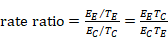 .
.
As a ratio measure, this rate ratio should then be log transformed for analysis (see Section 6.3.2). An approximate SE of the log rate ratio is given by:
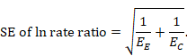
A correction of 0.5 may be added to each count in the case of zero events. Note that the choice of time unit (i.e. patient-months, woman-years, etc) is irrelevant since it is cancelled out of the rate ratio and does not figure in the SE. However, the units should still be displayed when presenting the study results.
It is also possible to use a rate difference (or difference in rates) as a summary statistic, although this is much less common:
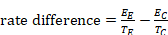 .
.
An approximate SE for the rate difference is:
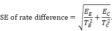
Counts of more common events, such as counts of decayed, missing or filled teeth, may often be treated in the same way as continuous outcome data. The intervention effect used will be the MD which will compare the difference in the mean number of events (possibly standardized to a unit time period) experienced by participants in the intervention group compared with participants in the comparator group.
6.7.2 Data extraction for counts and rates
Data that are inherently counts may have been analysed in several ways. Both primary investigators and review authors will need to decide whether to make the outcome of interest dichotomous, continuous, time-to-event or a rate (see Section 6.8).
Although it is preferable to decide how count data will be analysed in a review in advance, the choice often is determined by the format of the available data, and thus cannot be decided until the majority of studies have been reviewed. Review authors should plan to extract count data in the form in which they are reported.
Sometimes detailed data on events and person-years at risk are not available, but results calculated from them are. For example, an estimate of a rate ratio or rate difference may be presented. Such data may be included in meta-analyses only when they are accompanied by measures of uncertainty such as a 95% confidence interval (see Section 6.3), from which a SE can be obtained and the generic inverse variance method used for meta-analysis.
6.7.2.1 Extracting counts as dichotomous data
A common error is to attempt to treat count data as dichotomous data. Suppose that in the example just presented, the 18 MIs in 314 person-years arose from 157 patients observed on average for 2 years. One may be tempted to quote the results as 18/157, or even 18/314. This is inappropriate if multiple MIs from the same patient could have contributed to the total of 18 (say if the 18 arose through 12 patients having single MIs and 3 patients each having 2 MIs). The total number of events could theoretically exceed the number of patients, making the results nonsensical. For example, over the course of one year, 35 epileptic participants in a study could experience a total of 63 seizures.
To consider the outcome as a dichotomous outcome, the author must determine the number of participants in each intervention group, and the number of participants in each intervention group who experienced at least one event (or some other appropriate criterion which classified all participants into one of two possible groups). Any time element in the data is lost through this approach, though it may be possible to create a series of dichotomous outcomes, for example at least one stroke during the first year of follow-up, at least one stroke during the first two years of follow-up, and so on. It may be difficult to derive such data from published reports.
6.7.2.2 Extracting counts as continuous data
To extract counts as continuous data (i.e. the mean number of events per patient), guidance in Section 6.5.2 should be followed, although particular attention should be paid to the likelihood that the data will be highly skewed.
6.7.2.3 Extracting counts as time-to-event data
For rare events that can happen more than once, an author may be faced with studies that treat the data as time-to-first-event. To extract counts as time-to-event data, guidance in Section 6.8.2 should be followed.
6.7.2.4 Extracting counts as rate data
When it is possible to extract the total number of events in each group, and the total amount of person-time at risk in each group, then count data can be analysed as rates (see Chapter 10, Section 10.8). Note that the total number of participants is not required for an analysis of rate data but should be recorded as part of the description of the study.
6.8 Time-to-event data
6.8.1 Effect measures for time-to-event outcomes
Time-to-event data arise when interest is focused on the time elapsing before an event is experienced. They are known generically as survival data in the medical statistics literature, since death is often the event of interest, particularly in cancer and heart disease. Time-to-event data consist of pairs of observations for each individual: first, a length of time during which no event was observed, and second, an indicator of whether the end of that time period corresponds to an event or just the end of observation. Participants who contribute some period of time that does not end in an event are said to be ‘censored’. Their event-free time contributes information and they are included in the analysis. Time-to-event data may be based on events other than death, such as recurrence of a disease event (for example, time to the end of a period free of epileptic fits) or discharge from hospital.
Time-to-event data can sometimes be analysed as dichotomous data. This requires the status of all patients in a study to be known at a fixed time point. For example, if all patients have been followed for at least 12 months, and the proportion who have incurred the event before 12 months is known for both groups, then a 2✕2 table can be constructed (see Box 6.4.a) and intervention effects expressed as risk ratios, odds ratios or risk differences.
It is not appropriate to analyse time-to-event data using methods for continuous outcomes (e.g. using mean times-to-event), as the relevant times are only known for the subset of participants who have had the event. Censored participants must be excluded, which almost certainly will introduce bias.
The most appropriate way of summarizing time-to-event data is to use methods of survival analysis and express the intervention effect as a hazard ratio. Hazard is similar in notion to risk, but is subtly different in that it measures instantaneous risk and may change continuously (for example, one’s hazard of death changes as one crosses a busy road). A hazard ratio describes how many times more (or less) likely a participant is to suffer the event at a particular point in time if they receive the experimental rather than the comparator intervention. When comparing interventions in a study or meta-analysis, a simplifying assumption is often made that the hazard ratio is constant across the follow-up period, even though hazards themselves may vary continuously. This is known as the proportional hazards assumption.
6.8.2 Data extraction for time-to-event outcomes
Meta-analysis of time-to-event data commonly involves obtaining individual patient data from the original investigators, re-analysing the data to obtain estimates of the hazard ratio and its statistical uncertainty, and then performing a meta-analysis (see Chapter 26). Conducting a meta-analysis using summary information from published papers or trial reports is often problematic as the most appropriate summary statistics often are not presented.
Where summary statistics are presented, three approaches can be used to obtain estimates of hazard ratios and their uncertainty from study reports for inclusion in a meta-analysis using the generic inverse variance methods. For practical guidance, review authors should consult Tierney and colleagues (Tierney et al 2007).
The first approach can be used when trialists have analysed the data using a Cox proportional hazards model (or some other regression models for survival data). Cox models produce direct estimates of the log hazard ratio and its SE, which are sufficient to perform a generic inverse variance meta-analysis. If the hazard ratio is quoted in a report together with a confidence interval or P value, an estimate of the SE can be obtained as described in Section 6.3.
The second approach is to estimate the hazard ratio approximately using statistics computed during a log-rank analysis. Collaboration with a knowledgeable statistician is advised if this approach is followed. The log hazard ratio (experimental relative to comparator) is estimated by (O−E)/V, which has SE=1/√V, where O is the observed number of events on the experimental intervention, E is the log-rank expected number of events on the experimental intervention, O−E is the log-rank statistic and V is the variance of the log-rank statistic (Simmonds et al 2011).
These statistics sometimes can be extracted from quoted statistics and survival curves (Parmar et al 1998, Williamson et al 2002). Alternatively, use can sometimes be made of aggregated data for each intervention group in each trial. For example, suppose that the data comprise the number of participants who have the event during the first year, second year, etc, and the number of participants who are event free and still being followed up at the end of each year. A log-rank analysis can be performed on these data, to provide the O–E and V values, although careful thought needs to be given to the handling of censored times. Because of the coarse grouping the log hazard ratio is estimated only approximately. In some reviews it has been referred to as a log odds ratio (Early Breast Cancer Trialists’ Collaborative Group 1990). When the time intervals are large, a more appropriate approach is one based on interval-censored survival (Collett 1994).
The third approach is to reconstruct approximate individual participant data from published Kaplan-Meier curves (Guyot et al 2012). This allows reanalysis of the data to estimate the hazard ratio, and also allows alternative approaches to analysis of the time-to-event data.
6.9 Conditional outcomes only available for subsets of participants
Some study outcomes may only be applicable to a proportion of participants. For example, in subfertility trials the proportion of clinical pregnancies that miscarry following treatment is often of interest to clinicians. By definition this outcome excludes participants who do not achieve an interim state (clinical pregnancy), so the comparison is not of all participants randomized. As a general rule it is better to re-define such outcomes so that the analysis includes all randomized participants. In this example, the outcome could be whether the woman has a ‘successful pregnancy’ (becoming pregnant and reaching, say, 24 weeks or term). If miscarriage is the outcome of interest, then appropriate analysis can be performed using individual participant data, but is rarely possible using summary data. Another example is provided by a morbidity outcome measured in the medium or long term (e.g. development of chronic lung disease), when there is a distinct possibility of a death preventing assessment of the morbidity. A convenient way to deal with such situations is to combine the outcomes, for example as ‘death or chronic lung disease’.
Challenges arise when a continuous outcome (say a measure of functional ability or quality of life following stroke) is measured only on those who survive to the end of follow-up. Two unsatisfactory options are: (i) imputing zero functional ability scores for those who die (which may not appropriately represent the death state and will make the outcome severely skewed), and (ii) analysing the available data (which must be interpreted as a non-randomized comparison applicable only to survivors). The results of these analyses must be interpreted taking into account any disparity in the proportion of deaths between the two intervention groups. More sophisticated options are available, which may increasingly be applied by trial authors (Colantuoni et al 2018).
6.10 Chapter information
Editors: Julian PT Higgins, Tianjing Li, Jonathan J Deeks
Acknowledgements: This chapter builds on earlier versions of the Handbook. For details of previous authors and editors of the Handbook, see Preface. We are grateful to Judith Anzures, Mike Clarke, Miranda Cumpston, Peter Gøtzsche and Christopher Weir for helpful comments.
Funding: JPTH is a member of the National Institute for Health Research (NIHR) Biomedical Research Centre at University Hospitals Bristol NHS Foundation Trust and the University of Bristol. JJD received support from the NIHR Birmingham Biomedical Research Centre at the University Hospitals Birmingham NHS Foundation Trust and the University of Birmingham. JPTH received funding from National Institute for Health Research Senior Investigator award NF-SI-0617-10145. The views expressed are those of the author(s) and not necessarily those of the NHS, the NIHR or the Department of Health.
6.11 References
Abrams KR, Gillies CL, Lambert PC. Meta-analysis of heterogeneously reported trials assessing change from baseline. Statistics in Medicine 2005; 24: 3823–3844.
Ades AE, Lu G, Dias S, Mayo-Wilson E, Kounali D. Simultaneous synthesis of treatment effects and mapping to a common scale: an alternative to standardisation. Research Synthesis Methods 2015; 6: 96–107.
Agresti A. An Introduction to Categorical Data Analysis. New York (NY): John Wiley & Sons; 1996.
Anzures-Cabrera J, Sarpatwari A, Higgins JPT. Expressing findings from meta-analyses of continuous outcomes in terms of risks. Statistics in Medicine 2011; 30: 2967–2985.
Bland M. Estimating mean and standard deviation from the sample size, three quartiles, minimum, and maximum. International Journal of Statistics in Medical Research 2015; 4: 57–64.
Colantuoni E, Scharfstein DO, Wang C, Hashem MD, Leroux A, Needham DM, Girard TD. Statistical methods to compare functional outcomes in randomized controlled trials with high mortality. BMJ 2018; 360: j5748.
Collett D. Modelling Survival Data in Medical Research. London (UK): Chapman & Hall; 1994.
Deeks J. Are you sure that’s a standard deviation? (part 1). Cochrane News 1997a; 10: 11–12.
Deeks J. Are you sure that’s a standard deviation? (part 2). Cochrane News 1997b; 11: 11–12.
Deeks JJ, Altman DG, Bradburn MJ. Statistical methods for examining heterogeneity and combining results from several studies in meta-analysis. In: Egger M, Davey Smith G, Altman DG, editors. Systematic Reviews in Health Care: Meta-analysis in Context. 2nd edition ed. London (UK): BMJ Publication Group; 2001. pp. 285–312.
Deeks JJ. Issues in the selection of a summary statistic for meta-analysis of clinical trials with binary outcomes. Statistics in Medicine 2002; 21: 1575–1600.
Dubey SD, Lehnhoff RW, Radike AW. A statistical confidence interval for true per cent reduction in caries-incidence studies. Journal of Dental Research 1965; 44: 921–923.
Early Breast Cancer Trialists’ Collaborative Group. Treatment of Early Breast Cancer. Volume 1: Worldwide Evidence 1985–1990. Oxford (UK): Oxford University Press; 1990.
Follmann D, Elliott P, Suh I, Cutler J. Variance imputation for overviews of clinical trials with continuous response. Journal of Clinical Epidemiology 1992; 45: 769–773.
Friedrich JO, Adhikari N, Herridge MS, Beyene J. Meta-analysis: low-dose dopamine increases urine output but does not prevent renal dysfunction or death. Annals of Internal Medicine 2005; 142: 510–524.
Friedrich JO, Adhikari NK, Beyene J. The ratio of means method as an alternative to mean differences for analyzing continuous outcome variables in meta-analysis: a simulation study. BMC Medical Research Methodology 2008; 8: 32.
Furukawa TA, Barbui C, Cipriani A, Brambilla P, Watanabe N. Imputing missing standard deviations in meta-analyses can provide accurate results. Journal of Clinical Epidemiology 2006; 59: 7–10.
Guyot P, Ades AE, Ouwens MJ, Welton NJ. Enhanced secondary analysis of survival data: reconstructing the data from published Kaplan-Meier survival curves. BMC Medical Research Methodology 2012; 12: 9.
Higgins JPT, White IR, Anzures-Cabrera J. Meta-analysis of skewed data: combining results reported on log-transformed or raw scales. Statistics in Medicine 2008; 27: 6072–6092.
Hozo SP, Djulbegovic B, Hozo I. Estimating the mean and variance from the median, range, and the size of a sample. BMC Medical Research Methodology 2005; 5: 13.
Johnston BC, Thorlund K, Schünemann HJ, Xie F, Murad MH, Montori VM, Guyatt GH. Improving the interpretation of quality of life evidence in meta-analyses: the application of minimal important difference units. Health and Quality of Life Outcomes 2010; 8: 116.
Laupacis A, Sackett DL, Roberts RS. An assessment of clinically useful measures of the consequences of treatment. New England Journal of Medicine 1988; 318: 1728–1733.
MacLennan JM, Shackley F, Heath PT, Deeks JJ, Flamank C, Herbert M, Griffiths H, Hatzmann E, Goilav C, Moxon ER. Safety, immunogenicity, and induction of immunologic memory by a serogroup C meningococcal conjugate vaccine in infants: a randomized controlled trial. JAMA 2000; 283: 2795–2801.
Marinho VCC, Higgins JPT, Logan S, Sheiham A. Fluoride toothpaste for preventing dental caries in children and adolescents. Cochrane Database of Systematic Reviews 2003; 1: CD002278.
Parmar MKB, Torri V, Stewart L. Extracting summary statistics to perform meta-analyses of the published literature for survival endpoints. Statistics in Medicine 1998; 17: 2815–2834.
Sackett DL, Deeks JJ, Altman DG. Down with odds ratios! Evidence Based Medicine 1996; 1: 164–166.
Sackett DL, Richardson WS, Rosenberg W, Haynes BR. Evidence-Based Medicine: How to Practice and Teach EBM. Edinburgh (UK): Churchill Livingstone; 1997.
Simmonds MC, Tierney J, Bowden J, Higgins JPT. Meta-analysis of time-to-event data: a comparison of two-stage methods. Research Synthesis Methods 2011; 2: 139–149.
Sinclair JC, Bracken MB. Clinically useful measures of effect in binary analyses of randomized trials. Journal of Clinical Epidemiology 1994; 47: 881–889.
Tierney JF, Stewart LA, Ghersi D, Burdett S, Sydes MR. Practical methods for incorporating summary time-to-event data into meta-analysis. Trials 2007; 8.
Vickers AJ. The use of percentage change from baseline as an outcome in a controlled trial is statistically inefficient: a simulation study. BMC Medical Research Methodology 2001; 1: 6.
Walter SD, Yao X. Effect sizes can be calculated for studies reporting ranges for outcome variables in systematic reviews. Journal of Clinical Epidemiology 2007; 60: 849–852.
Wan X, Wang W, Liu J, Tong T. Estimating the sample mean and standard deviation from the sample size, median, range and/or interquartile range. BMC Medical Research Methodology 2014; 14: 135.
Weir CJ, Butcher I, Assi V, Lewis SC, Murray GD, Langhorne P, Brady MC. Dealing with missing standard deviation and mean values in meta-analysis of continuous outcomes: a systematic review. BMC Medical Research Methodology 2018; 18: 25.
Williamson PR, Smith CT, Hutton JL, Marson AG. Aggregate data meta-analysis with time-to-event outcomes. Statistics in Medicine 2002; 21: 3337–3351.